The affected vendor did not answer to my responsible disclosure request, so I’m here to disclose this “hack” without revealing the name of the vendor itself.
The target machine uses an insecure NFC Card, MIFARE Classic 1k, that has been affected by multiple vulnerabilities so should not be used in important application.
Furthermore, the user’s credit was stored on the card enabling different attack scenarios, from double spending to potential data tamper storing an arbitrary credit.
Useful notes from MIFARE Classic 1K datasheet:
EEPROM: 1 kB is organized in 16 sectors of 4 blocks. One block contains 16 bytes.
The last block of each sector is called “trailer”, which contains two secret keys and programmable access conditions for each block in this sector.
- Manufacturer block: This is the first data block (block 0) of the first sector (sector 0). It contains the IC manufacturer data. This block is read-only.
- Data blocks: All sectors contain 3 blocks of 16 bytes for storing data (Sector 0 contains only two data blocks and the read-only manufacturer block).
The data blocks can be configured by the access conditions bits as:- Read/Write blocks: fully arbitrary data, in arbitrary format
- Value blocks: fixed data format which permits native error detection and correction and a backup management.
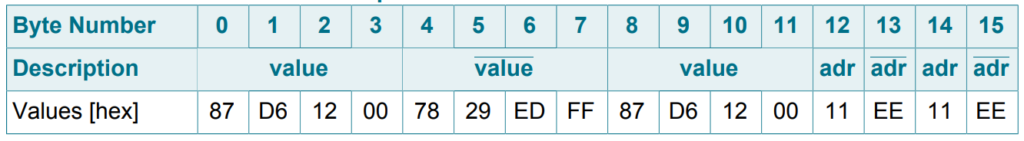
A value block can only be generated through a write operation in value block format:- Value: Signifies a signed 4-byte value. The lowest significant byte of a value is stored in the lowest address byte. Negative values are stored in standard 2´s complement format. For reasons of data integrity and security, a value is stored three times, twice non-inverted and once inverted.
- Adr: Signifies a 1-byte address, which can be used to save the storage address of a block, when implementing a powerful backup management. The address byte is stored four times, twice inverted and non-inverted.
Let’s start hacking:
In this post I did not show you how to crack the MIFARE Classic Keys needed to read/write the card, ’cause someone else has already disclosed it some time ago, so google is your friend.
At last, please, use this post to skill yourself about the fascinating world of reverse engineering, and not for stealing stuffs.
In order to start the analysis I need some dump to compare.
The requirements of this task are nfc-mfclassic tool included in libnfc, a NFC hardware interface like ACR122U, and a binary compare (aka binarydiff) tool like dhex.
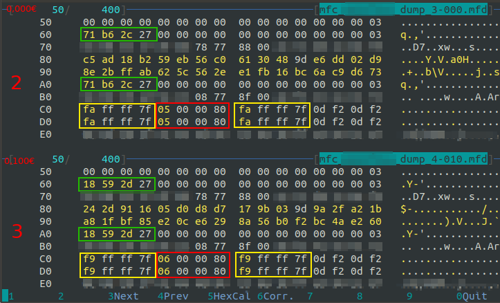
Dumps:
- Dump 0: Virgin card (not included in the screenshot below ’cause all data bytes were 0x00, except for the sector 0 that has UID and manufacturer information. These sector is read only, so these bytes are the same across dumps)
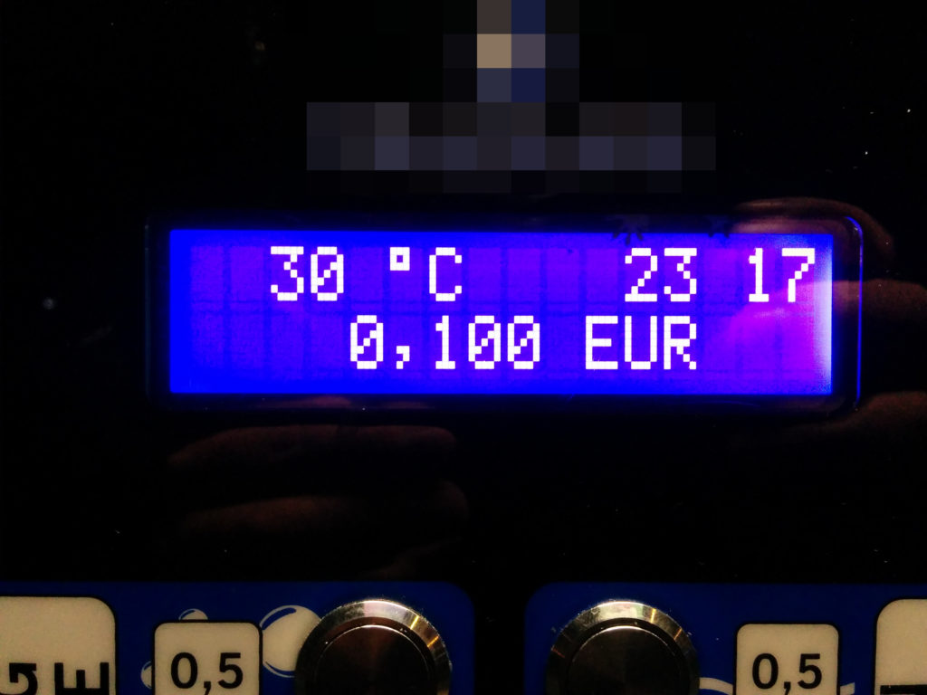
- Dump 1: Card charged with single 0.10€ coin (Note that vending machine displays the balance with 3 decimals, 0.100€)
- Dump 2: 0.00€ after spending the entire balance with 4 transactions of 0.025€ each
- Dump 3: 0.10€ recharged with one single coin
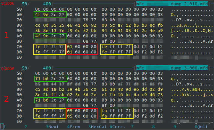
Blurred bytes are the MIFARE keys A and B, except for the 32 bytes at 0xE0 offset of which I don’t know their purpose.
The 4 bytes between the keys are Access Condition and denotes which key must be used for read and write operation (A or B key) and the block type (“read/write block” or “value block”).
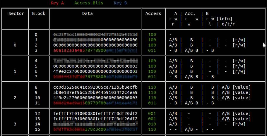
The tool mfdread is useful to decode the Access Condition bytes rapidly, and, in general, to display MIFARE Classic data divided by sectors and blocks:
Early analysis:
Note: from now on I will refer to the offsets with a [square parenthesis] and a value with no parenthesis.
- Blocks 8, 9, 10, 12 and 13 can be used also as “value block”
- Except for bytes between offsets [0x80] and [0x9F], only few bytes differ between dumps
- Some data are redundant, for example [0x60 … 0x63] has the same values of [0xA0 … 0xA3]
- Values at [0xC0], [0xD0], [0xC8], [0xD8] differ by 4 between 1st and 2nd dump (eg: 0xFE – 0xFA = 0x4) and differ by 1 between 2nd dump and 3rd dump (eg: 0xFA – 0xF9 = 0x1)
- Values at [0xC4], [0xD4] differ by 4 between 1st and 2nd dump (eg: 0x05 – 0x01 = 0x4) and differ by 1 between 2nd and 3rd dump (eg: 0x06 – 0x05 = 0x1)
- 4 is the number of spent transaction made the first time, and 1 is the number of recharge transaction made the second time
- Sum between yellow squared and red squared offsets has 0xFF value. In other words red squared is inverse (XOR with 0xFF) of yellow squared. For example:
- 0xFE ⊕ 0xFF = 0x01
- 0xFF ⊕ 0xFF = 0x00
- …
- 0x7F ⊕ 0xFF = 0x80
- Values at [0x60 … 0x63] are a UNIX TIMESTAMP in little endian notation:
- Dump 1: 0x4F9E2C27 -> 0x272C9E4F = 657235535 = 10/29/1990 @ 9:25pm
- Dump 2: 0x71B62C27 -> 0x272CB671 = 657241713 = 10/29/1990 @ 11:08pm
- Dump 3: 0x18592D27 -> 0x272D5918 = 657283352 = 10/30/1990 @ 10:42am
- Ok, we are not in the 90ies, but the time difference between transactions is correct, maybe the vending machine doesn’t have an UPS 🙂
Early findings:
- Timestamp of the last transaction was stored as 32 bit integer at MIFARE block 6 and redundant at at MIFARE block 10
- Only MIFARE blocks 12 and 13 has “Value block” format, and they are used to store the counter of remain transaction in 32 bit format.
This counter starts from 0x7FFFFFFF (2.147.483.647) and is decreased at each transaction - Blocks 1, 4, and 14 contains some data that are fixed between dumps
- Blocks 8 and 9 changes entirely at each transaction
The credit:
If there is credit stored on the card, it was encoded at blocks 8 and 9, and the number of bytes involved between small credit difference (for example between 0.00€ and 0.10€) could indicate that some cryptographic function is involved.
At this time, a double spending attack could confirm if the credit is really stored on the card.
So, after spending all the credit, I have rewritten a previous dump on the card and I went to test it at the vending machine. The card was fully functional with the previous credit stored in that dump. Now, I’m certain that the credit is encoded (and probably encrypted) in the blocks 8 and 9.
Conclusion:
Even if the encoding format of the credit is still unknown, a double spending attack was possible.
This means that the vendor’s effort to obfuscate the credit is nullified 🙁
Adding some unique token on the card that are invalidated into back-end after each transaction, means that this token needs to be shared between all the vending machines of the vendor, but, if we add internet connection to the vending machine, there is no longer reason to store the credit on the card.
So, after all, the only remediation action that makes sense is: DO NOT STORE THE CREDIT ON THE CARD! And, more generally: DO NOT TRUST THE CLIENT!
Road to arbitrary credit:
Spending 1€ infinite times isn’t the scope of that hack. The only real scope is FUN!
To continue this analysis I need to collect a large number of dumps to advance some hypothesis so, when I have other material I will make another post.
An example of easier card:
Some vendor has more easier approach by using the MIFARE “Value block” to store the credit without obfuscation or encryption.
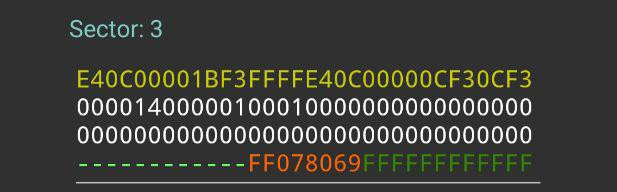
The above screenshot made with “MIFARE Classic Tool” on Android smartphone, represents a Value Block used to store the credit:
0x00000CE4 = 3300 is the value in Euro thousandths (3.30€).
This particular vendor do not use key A and the Key B is a default key 0xFFFFFFFFFFFFFFFF, so the attacker doesn’t need to crack anything.
Reverse engineering and cracking of a Vending Machine is always funny 🙂